GeoTiff data component
The GeoTiff data component, pymt_geotiff, is a Python Modeling Toolkit (pymt) library for accessing data (and metadata) from a GeoTIFF file, through either a local filepath or a remote URL.
The pymt_geotiff component provides BMI-mediated access to GeoTIFF data as a service, allowing them to be coupled in pymt with other data or model components that expose a BMI.
Installation
pymt, and components that run within it, are distributed through Anaconda and the conda package manager. Instructions for installing Anaconda can be found on their website. In particular, pymt components are available through the community-led conda-forge organization.
Install the pymt and pymt_geotiff packages in a new environment with:
$ conda create -n pymt -c conda-forge python=3 pymt pymt_geotiff
$ conda activate pymt
conda automatically resolves and installs any required dependencies.
Use
The pymt_geotiff data component is designed to access data in a GeoTIFF file, with the user providing the location of the file through either a filepath or an URL. This information can be provided through a configuration file or specified through parameters.
With a configuration file
The pymt_geotiff configuration file is a YAML file
containing keys that map to parameter names.
An example is bmi-geotiff.yaml:
bmi-geotiff:
  filename: https://github.com/mapbox/rasterio/raw/master/tests/data/RGB.byte.tif
Download this file
for use in the following example.
Start by importing the GeoTiff class from pymt.
from pymt.models import GeoTiff
Create an instance.
m = GeoTiff()
In this case, we’ll initialize the GeoTiff component with information from a configuration file. (This may take a moment as data are fetched from the internet.)
m.initialize("bmi-geotiff.yaml")
Note that the configurtation information has been read from the configuration file into the component as parameters.
What variables can be accessed from this component?
for var in m.output_var_names:
    print(var)
gis__raster_data
gis__coordinate_reference_system
gis__gdal_geotransform
Get the GDAL GeoTransform used by the data.
m.var["gis__gdal_geotransform"].data
array([  3.00037927e+02,   0.00000000e+00,   1.01985000e+05,
         0.00000000e+00,  -3.00041783e+02,   2.82691500e+06])
What are the units of the transformation?
m.var["gis__gdal_geotransform"].units
'm'
Finish by finalizing the component.
m.finalize()
With parameters
Configuration information can also be passed directly to pymt_geotiff as parameters.
Start by importing the GeoTiff class from pymt and creating an
instance.
from pymt.models import GeoTiff
m = GeoTiff()
Next, use the setup method to assign values to the parameters needed by GeoTiff.
args = m.setup(
    "test",
    filename="https://github.com/mapbox/rasterio/raw/master/tests/data/RGB.byte.tif",
)
Pass the results from setup into the initialize method. (This step may take a moment as data are fetched from the internet.)
m.initialize(*args)
*** <xarray.Rectilinear>
Dimensions:     (rank: 3)
Dimensions without coordinates: rank
Data variables:
    mesh        int64 0
    node_shape  (rank) int32 3 718 791
Note that the parameters have been correctly assigned in the component:
for param in m.parameters:
    print(param)
('filename', 'https://github.com/mapbox/rasterio/raw/master/tests/data/RGB.byte.tif')
What variables can be accessed from this component?
for var in m.output_var_names:
    print(var)
gis__raster_data
gis__coordinate_reference_system
gis__gdal_geotransform
Get the raster data values.
raster = m.var["gis__raster_data"].data
Let’s visualize these data.
The pymt_geotiff component contains not only data values, but also the grid on which they’re located. Start by getting the identifier for the grid used for the raster data.
gid = m.var_grid("gis__raster_data")
Using the grid identifier, we can get the grid dimensions and the locations of the grid nodes.
shape = m.grid_shape(gid)
x = m.grid_x(gid)
y = m.grid_y(gid)
print("shape:", shape)
print("x:", x)
print("y:", y)
shape: [  3 718 791]
x: [ 102135.01896334  102435.05689001  102735.09481669  103035.13274336
  ...
  338564.90518331  338864.94310999  339164.98103666]
y: [ 2826764.97910863  2826464.93732591  2826164.89554318  2825864.85376045
  ...
  2611935.06267409  2611635.02089137]
We’re almost ready to make a plot. Note, however, that the default
behavior of pymt components is to flatten data arrays.
raster.shape
(1703814,)
Make a new variable that restores the dimensionality of the data.
raster3D = raster.reshape(shape)
raster3D.shape
(3, 718, 791)
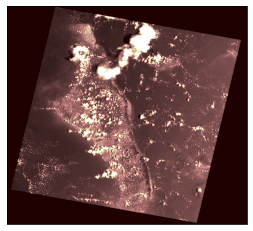
Extract the red band from the image.
red_band = raster3D[0,:,:]
red_band.shape
(718, 791)
What information do we have about how the data are projected?
projection = m.var["gis__coordinate_reference_system"].data
projection
array(['+init=epsg:32618'],
      dtype='<U16')
transform = m.var["gis__gdal_geotransform"].data
transform
array([  3.00037927e+02,   0.00000000e+00,   1.01985000e+05,
         0.00000000e+00,  -3.00041783e+02,   2.82691500e+06])
We’ll use cartopy to help display the data in a map projection.
import cartopy.crs as ccrs
The data are in UTM zone 18N, but the projection must be set manually. (A note in the xarray documentation describes this.)
crs = ccrs.UTM('18N')
Display the red band of the image in the appropriate projection.
import matplotlib.pyplot as plt

ax = plt.subplot(projection=crs)
ax.imshow(red_band, transform=crs, extent=[x.min(),x.max(),y.min(),y.max()], cmap="pink")
<matplotlib.image.AxesImage at 0x1a23b4be0>
Complete the example by finalizing the component.
m.finalize()
API documentation
Looking for information on a particular function, class, or method? This part of the documentation is for you.
Help
Depending on your need, CSDMS can provide advice or consulting services. Feel free to contact us through the CSDMS Help Desk.
Acknowledgments
This work is supported by the National Science Foundation under Award No. 1831623, Community Facility Support: The Community Surface Dynamics Modeling System (CSDMS).